4.2. Counterfactual predictions for impact variables

This section provides more details on the way counterfactual predictions are carried out by eensight for events that affect impact variables, such as an energy retrofit. To this end, it outlines the methodology behind the predict and evaluate pipelines of eensight.

%load_ext autoreload
%autoreload 2

from datetime import time

import pandas as pd
import matplotlib.patches as mpatches
import matplotlib.pyplot as plt
import matplotlib.ticker as ticker

from eensight.config import ConfigLoader
from eensight.methods.prediction.baseline import UsagePredictor
from eensight.methods.prediction.activity import estimate_activity
from eensight.methods.prediction.metrics import cvrmse, nmbe
from eensight.settings import PROJECT_PATH
from eensight.utils import get_categorical_cols, load_catalog

plt.style.use("bmh")

%matplotlib inline

4.2.1. The b02 dataset

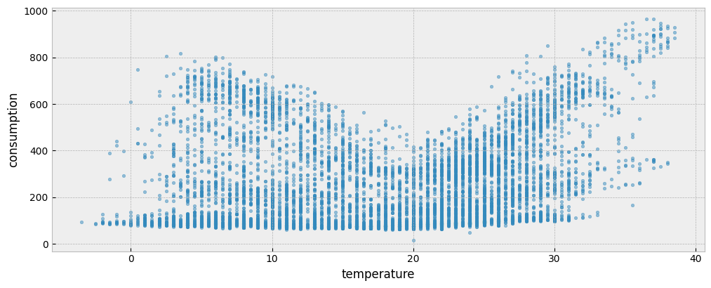
The b02 dataset corresponds to the building with id=13 of the dataset provided by the EnergyDetective 2020 competition.

Start with the train data:

catalog_train = load_catalog(store_uri="../../../data", site_id="b02", namespace="train")

X_train = catalog_train.load("train.preprocessed-features")
y_train = catalog_train.load("train.preprocessed-labels")

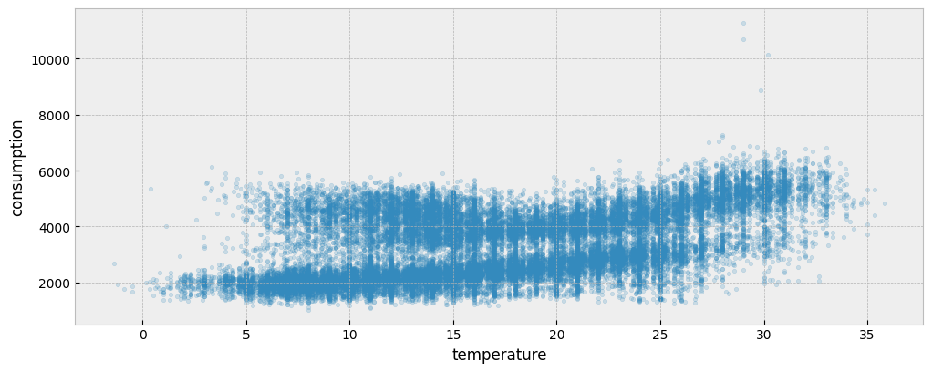
The following plot presents the energy consumption of the selected dataset as a function of the outdoor temperature:

fig = plt.figure(figsize=(12, 4.5))
layout = (1, 1)
ax = plt.subplot2grid(layout, (0, 0))

ax.scatter(X_train["temperature"], y_train["consumption"], s=10, alpha=0.5)
ax.set_xlabel("temperature")
ax.set_ylabel("consumption")

4.2.2. The predict pipeline

The predict pipeline performs the following steps:

When run in the train namespace

Fits a predictive model on the train data using the eensight.methods.prediction.baseline.UsagePredictor model. We don’t need to add calendar features, since the UsagePredictor adds calendar features as needed:

model = UsagePredictor().fit(X_train, y_train)

The predict pipeline can be called from the command line as:

eensight run predict --site-id b02 --store-uri ../../../data --namespace train 

Running the pipeline will create the following artifacts:

• model: The trained UsagePredictor model

• train.prediction: A dataframe with the prediction generated by applying the model on the train data (in-sample prediction)

• train.performance: A JSON file with the in-sample CV(RMSE) and NMBE.

When run in the test namespace

Load the test data:

catalog_test = load_catalog(store_uri="../../../data", site_id="b02", namespace="test")

X_test = catalog_test.load("test.preprocessed-features")
y_test = catalog_test.load("test.preprocessed-labels")

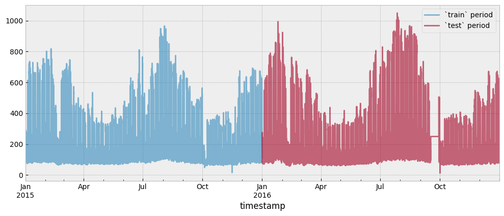
Both the train and test period consumption data are presented in the next plot:

fig = plt.figure(figsize=(12, 4.5))
layout = (1, 1)
ax = plt.subplot2grid(layout, (0, 0))

y_train.plot(ax=ax, alpha=0.6)
y_test.plot(ax=ax, alpha=0.6)
ax.legend(["`train` period", "`test` period"], frameon=True)

Apply the model on the test data:

prediction = model.predict(X_test)

The Coefficient of Variation of the Root Mean Squared Error CV(RMSE) is:

cvrmse(y_test, prediction)

0.3042765589248083

The Normalized Mean Bias Error (NMBE) is:

nmbe(y_test, prediction)

0.007393580383622497

The UsagePredictor model allows us to add time lags for selected features. If we want to add 1-hour, 2-hour and 24-hour time lags for temperature, we can write:

lags = {"temperature": [1, 2, 24]}

model = UsagePredictor(lags=lags).fit(X_train, y_train)

Adding time lags may improve the accuracy of the model:

prediction = model.predict(X_test)
cvrmse(y_test, prediction)

0.29944357827501156

nmbe(y_test, prediction)

0.005027632126261972

The predict pipeline can be called from the command line as:

eensight run predict --site-id b02 --store-uri ../../../data --namespace test 

Running the pipeline will create the following artifacts:

• test.prediction: A dataframe with the prediction generated by applying the model on the test data (out-of-sample prediction)

To actually get the metrics for the predictive performance of the model, we have to call the evaluate pipeline:

eensight run evaluate --site-id b02 --store-uri ../../../data --namespace test 

Running the pipeline will create the following artifacts:

• test.performance: A JSON file with the out-of-sample CV(RMSE) and NMBE.

Note that:

1. The predict pipeline must be called first in the train namespace and, then, in the test one, so that the model is available.

2. The predict pipeline must be called before the evaluate, so that the test.prediction is available to the latter.

3. The evaluate pipeline supports only the test and apply namespaces.

When run in the apply namespace

We can use the fitted model to carry out a counterfactual prediction for the apply period:

catalog_apply = load_catalog(store_uri="../../../data", site_id="b02", namespace="apply")

X_apply = catalog_apply.load("apply.preprocessed-features")
y_apply = catalog_apply.load("apply.preprocessed-labels")

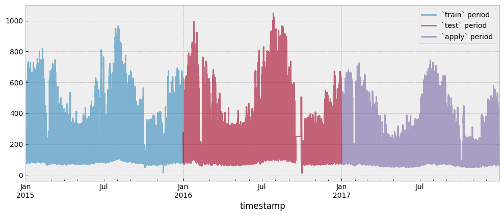
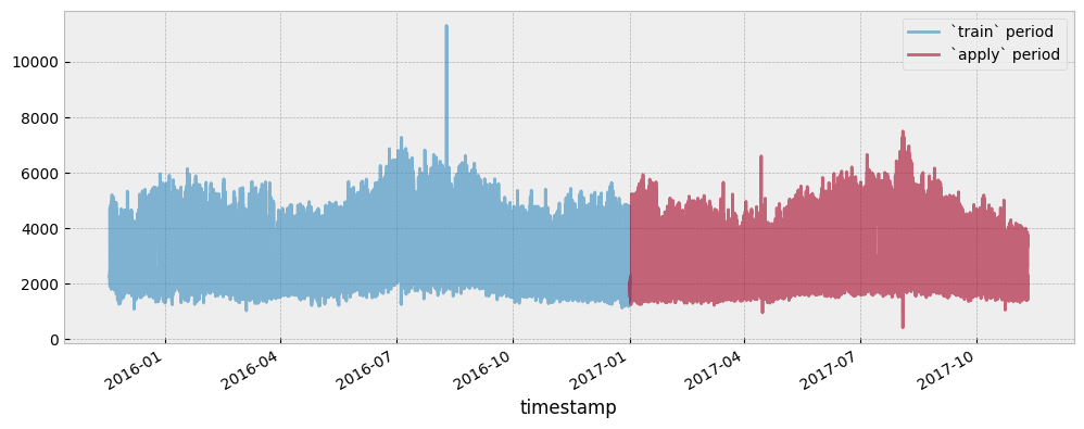
The train, test and apply period consumption data are presented in the next plot:

fig = plt.figure(figsize=(12, 4.5))
layout = (1, 1)
ax = plt.subplot2grid(layout, (0, 0))

y_train.plot(ax=ax, alpha=0.6)
y_test.plot(ax=ax, alpha=0.6)
y_apply.plot(ax=ax, alpha=0.6)

ax.legend(["`train` period", "`test` period", "`apply` period"], frameon=True)

Evaluate the model on the apply data:

prediction = model.predict(X_apply)

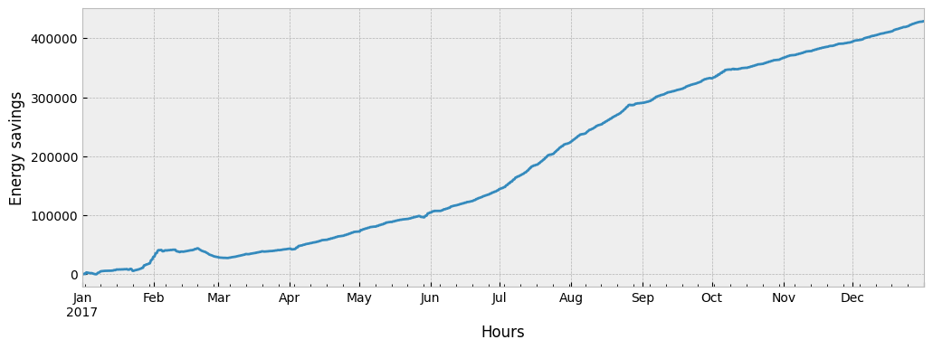
Since train and apply data are separated by an event (train is pre-event data and apply is post-event), the difference between the predicted and the actual energy consumption is an estimation of the event’s impact.

impact = prediction - y_apply["consumption"]

Typically, the impact (expressed in this case as energy savings) is visualized as a cumulative variable:

fig = plt.figure(figsize=(12, 4))
layout = (1, 1)
ax = plt.subplot2grid(layout, (0, 0))

impact.cumsum().plot(ax=ax)

ax.set_xlabel('Hours')
ax.set_ylabel('Energy savings')

The predict pipeline can be called from the command line as:

eensight run predict --site-id b02 --store-uri ../../../data --namespace apply 

Running the pipeline will create the following artifacts:

• apply.prediction: A dataframe with the prediction generated by applying the model on the apply data (counterfactual prediction)

To actually get the impact estimation, we have to call the evaluate pipeline:

eensight run evaluate --site-id b02 --store-uri ../../../data --namespace apply 

Running the pipeline will create the following artifacts:

• apply.impact: A dataframe with the difference between the predicted and the actual energy consumption.

Note that the predict pipeline must be called before the evaluate, so that the apply.prediction is available to the latter.

In practice, the predicitive model can be used for generating counterfactual energy consumption predictions until we observe enough data in the reporting period. When enough data is available, we can run the predict pipeline with the flag --autoencode.

In this case:

4.2.3. The predict pipeline with autoencoding

When run in the train namespace

First, estimate activity levels.

for feature in X_train.columns:
    print(feature)

temperature
dew point temperature
relative humidity
atmospheric pressure
wind speed

non_occ_features = [
    "temperature",
    "dew point temperature",
    "relative humidity",
    "atmospheric pressure",
    "wind speed"
]

act_train = estimate_activity(
    X_train, 
    y_train, 
    non_occ_features=non_occ_features, 
    exog="temperature",
    n_trials=200,
    verbose=False,
)

Then, fit a predictive model for the train data using the activity estimation as a feature. In this case, we set the UsagePredictor’s parameter skip_calendar to True, so that calendar features are not generated automatically:

X_train_act = pd.concat(
    [
        X_train,
        act_train.to_frame("activity")
        
    ], 
    axis=1
)

model_autoenc = UsagePredictor(lags=lags, skip_calendar=True).fit(X_train_act, y_train)

The predict pipeline can be called from the command line as:

eensight run predict --site-id b02 --store-uri ../../../data --namespace train --autoencode

Running the pipeline will create the following artifacts:

• train.activity: Dataframe with the estimated activity levels for the train data.

• model-autoenc: The trained UsagePredictor model using activity levels as a feature.

• train.prediction-autoenc: A dataframe with the prediction generated by applying model-autoenc on the train data.

• train.performance-autoenc: A JSON file with the CV(RMSE) and NMBE.

When run in the test namespace

Estimate activity levels:

act_test = estimate_activity(
    X_test, 
    y_test, 
    non_occ_features=non_occ_features, 
    exog="temperature",
    n_trials=200,
    verbose=False,
)

Use the model that was fitted on the train data to predict energy consumption:

X_test_act = pd.concat(
    [
        X_test,
        act_test.to_frame("activity")
    ], 
    axis=1
)

prediction = model_autoenc.predict(X_test_act)

Autoencoding improves predictive accuracy on test data, but not in a drastic way that would indicate overfitting due to data leakage:

cvrmse(y_test, prediction)

0.2805189614516902

nmbe(y_test, prediction)

0.03583116402388926

The predict pipeline can be called from the command line as:

eensight run predict --site-id b02 --store-uri ../../../data --namespace test --autoencode

Running the pipeline will create the following artifacts:

• test.activity: Dataframe with the estimated activity levels for the test data.

• test.prediction-autoenc: A dataframe with the prediction generated by applying model-autoenc on the test data

To actually get the metrics for the predictive performance of the model, we have to call the evaluate pipeline:

eensight run evaluate --site-id b02 --store-uri ../../../data --namespace test --autoencode

Running the pipeline will create the following artifacts:

• test.performance-autoenc: A JSON file with the CV(RMSE) and NMBE values.

Note that the predict pipeline must be called before the evaluate, so that the test.prediction-autoenc is available to the latter.

When run in the apply namespace

Estimate activity levels:

act_apply = estimate_activity(
    X_apply, 
    y_apply, 
    non_occ_features=non_occ_features, 
    exog="temperature",
    n_trials=200,
    verbose=False,
)

If the predict pipeline runs on the apply data, the consumption model generates a counterfactual prediction:

X_counter = pd.concat(
    [
        X_apply,
        act_apply.to_frame("activity")
    ], 
    axis=1
)

prediction = model_autoenc.predict(X_counter)

impact_autoenc = prediction - y_apply["consumption"]

The predict pipeline can be called from the command line as:

eensight run predict --site-id b02 --store-uri ../../../data --namespace apply --autoencode

Running the pipeline will create the following artifacts:

• apply.activity: Dataframe with the estimated activity levels for the apply data.

• apply.prediction-autoenc: A dataframe with the prediction generated by applying model-autoenc on the apply data.

To actually get the impact estimation, we have to call the evaluate pipeline:

eensight run evaluate --site-id b02 --store-uri ../../../data --namespace apply --autoencode

Running the pipeline will create the following artifacts:

• apply.impact-autoenc: A dataframe with the difference between the predicted and the actual energy consumption.

Note that the predict pipeline must be called before the evaluate, so that the apply.prediction-autoenc is available to the latter.

We can compare the estimated impact from the two approaches:

fig = plt.figure(figsize=(12, 4))
layout = (1, 1)
ax = plt.subplot2grid(layout, (0, 0))

impact.cumsum().plot(ax=ax)
impact_autoenc.cumsum().plot(ax=ax)

ax.set_xlabel('Hours')
ax.set_ylabel('Energy savings')
ax.legend(["Impact estimation", "Updated impact estimation"], frameon=True)

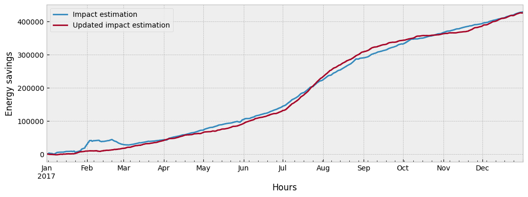
What drives the difference between the two impact estimations and which one should we trust more?

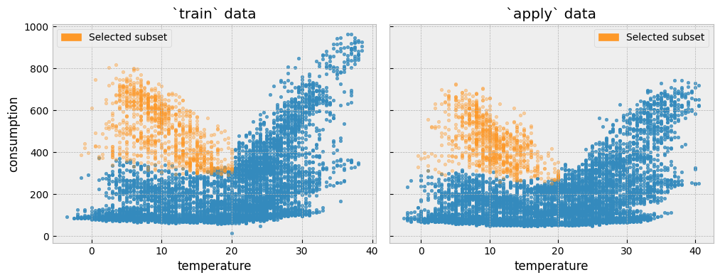
Let’s isolate all train and apply observations where temperature is lower than 20\(^{\circ}C\) and activity equals one (1):

low_temp_periods_train = X_train[X_train["temperature"] <= 20].index

y_train_selected = y_train[
    y_train.index.isin(low_temp_periods_train) 
    & y_train.index.isin(act_train[act_train == 1].index)
]

low_temp_periods_apply = X_apply[X_apply["temperature"] <= 20].index

y_apply_selected = y_apply[
    y_apply.index.isin(low_temp_periods_apply) 
    & y_apply.index.isin(act_apply[act_apply == 1].index)
]

We can plot the two subsets side by side:

fig, (ax1, ax2) = plt.subplots(1, 2, sharey=True, figsize=(12, 4))
fig.subplots_adjust(wspace=0.04)

ax1.scatter(
    X_train.loc[~X_train.index.isin(y_train_selected.index), "temperature"], 
    y_train.loc[~y_train.index.isin(y_train_selected.index), "consumption"], 
    s=10, 
    alpha=0.8
)

ax1.scatter(
    X_train.loc[y_train_selected.index, "temperature"], 
    y_train_selected["consumption"], 
    s=10, 
    alpha=0.4,
    color="#fe9929"
)

ax1.set_xlabel("temperature")
ax1.set_ylabel("consumption")
ax1.set_title("`train` data")

ax1.legend(
    handles=[
        mpatches.Patch(color="#fe9929", label="Selected subset"), 
    ]
)

ax2.scatter(
    X_apply.loc[~X_apply.index.isin(y_apply_selected.index), "temperature"], 
    y_apply.loc[~y_apply.index.isin(y_apply_selected.index), "consumption"],
    s=10, 
    alpha=0.8
)

ax2.scatter(
    X_apply.loc[y_apply_selected.index, "temperature"], 
    y_apply_selected["consumption"], 
    s=10, 
    alpha=0.4,
    color="#fe9929"
)

ax2.set_xlabel("temperature")
ax2.set_title("`apply` data")

ax2.legend(
    handles=[
        mpatches.Patch(color="#fe9929", label="Selected subset"), 
    ]
)

First, we will plot the distribution of the actual energy consumption for the selected train and the apply observations:

fig = plt.figure(figsize=(12, 4))
layout = (1, 1)
ax = plt.subplot2grid(layout, (0, 0))

y_train_selected.plot.kde(ax=ax, color="#034e7b")
y_apply_selected.plot.kde(ax=ax, color="#cc4c02")

selected_train_average = y_train_selected["consumption"].mean()
selected_apply_average = y_apply_selected["consumption"].mean()

ax.axvline(x=selected_train_average, color="#034e7b", ls=":")
ax.axvline(x=selected_apply_average, color="#cc4c02", ls=":")

ax.annotate(
    f"Average change: {round(selected_apply_average - selected_train_average, 2)}", 
    xy=(490, 0.001), 
    xytext=(150, 0.0032), 
    arrowprops={"arrowstyle":"->", "color":"black"}
)

ax.legend(["`train` data", "`apply` data"], frameon=True)

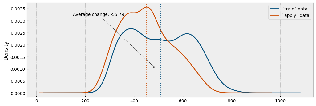
This is pretty much how a counterfactual prediction should work: find similar conditions between the pre- and post-event data (here, similar temperature and activity levels), and compare the difference in the energy consumption.

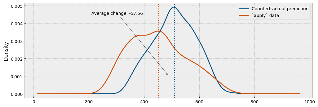
Next, we will estimate the energy consumption using the predictive model and compare the predicted with the actual consumption:

X_apply_selected = X_apply.loc[y_apply_selected.index]

prediction = model.predict(X_apply_selected)

fig = plt.figure(figsize=(12, 4))
layout = (1, 1)
ax = plt.subplot2grid(layout, (0, 0))

prediction.plot.kde(ax=ax, color="#034e7b")
y_apply_selected.plot.kde(ax=ax, color="#cc4c02")

prediction_average = prediction.mean()
selected_apply_average = y_apply_selected["consumption"].mean()

ax.axvline(x=prediction_average, color="#034e7b", ls=":")
ax.axvline(x=selected_apply_average, color="#cc4c02", ls=":")

ax.annotate(
    f"Average change: {round(selected_apply_average - prediction_average, 2)}", 
    xy=(450, 0.001), 
    xytext=(150, 0.0035), 
    arrowprops={"arrowstyle":"->", "color":"black"}
)

ax.legend(["Counterfractual prediction", "`apply` data"], frameon=True)

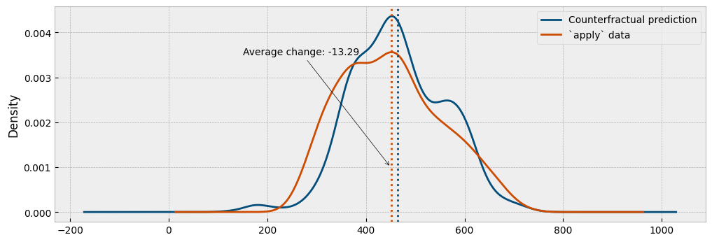
Finally, we will estimate the energy consumption using the autoencoding model and compare the predicted with the actual consumption:

X_counter = pd.concat(
    [
        X_apply_selected,
        act_apply.loc[X_apply_selected.index].to_frame("activity")
    ], 
    axis=1
)

prediction = model_autoenc.predict(X_counter)

fig = plt.figure(figsize=(12, 4))
layout = (1, 1)
ax = plt.subplot2grid(layout, (0, 0))

prediction.plot.kde(ax=ax, color="#034e7b")
y_apply_selected.plot.kde(ax=ax, color="#cc4c02")

prediction_average = prediction.mean()
selected_apply_average = y_apply_selected["consumption"].mean()

ax.axvline(x=prediction_average, color="#034e7b", ls=":")
ax.axvline(x=selected_apply_average, color="#cc4c02", ls=":")

ax.annotate(
    f"Average change: {round(selected_apply_average - prediction_average, 2)}", 
    xy=(490, 0.001), 
    xytext=(210, 0.0045), 
    arrowprops={"arrowstyle":"->", "color":"black"}
)

ax.legend(["Counterfractual prediction", "`apply` data"], frameon=True)

As we can see from the plots, the autoencoding approach provides a generally better representation of the actual impact.

4.2.4. The b03 dataset

The b03 data corresponds to the building with id=50 from the dataset of the Power Laws: Forecasting Energy Consumption competition.

Start with the train data:

catalog_train = load_catalog(store_uri="../../../data", site_id="b03", namespace="train")

X_train = catalog_train.load("train.preprocessed-features")
y_train = catalog_train.load("train.preprocessed-labels")

The following plot presents the energy consumption of the selected dataset as a function of the outdoor temperature:

fig = plt.figure(figsize=(12, 4.5))
layout = (1, 1)
ax = plt.subplot2grid(layout, (0, 0))

ax.scatter(X_train["temperature"], y_train["consumption"], s=10, alpha=0.2)
ax.set_xlabel("temperature")
ax.set_ylabel("consumption")

4.2.5. The predict pipeline

When run in the train namespace

Fit a predictive model on the train data using the UsagePredictor model. Note that there is one categorical feature in the data:

get_categorical_cols(X_train, int_is_categorical=False)

['holiday']

model = UsagePredictor(cat_features="holiday").fit(X_train, y_train)

When run in the apply namespace

Load the apply data:

catalog_apply = load_catalog(store_uri="../../../data", site_id="b03", namespace="apply")

X_apply = catalog_apply.load("apply.preprocessed-features")
y_apply = catalog_apply.load("apply.preprocessed-labels")

Both the train and apply period consumption data are presented in the next plot:

fig = plt.figure(figsize=(12, 4.5))
layout = (1, 1)
ax = plt.subplot2grid(layout, (0, 0))

y_train.plot(ax=ax, alpha=0.6)
y_apply.plot(ax=ax, alpha=0.6)
ax.legend(["`train` period", "`apply` period"], frameon=True)

Evaluate the model on the apply data:

prediction = model.predict(X_apply)

For this dataset, there is a time shift in the daily profiles between the train and the apply data. This time shift can be spotted when directly comparing the train and apply daily profiles:

y_train_daily = y_train.copy()
y_train_daily["date"] = y_train_daily.index.date
y_train_daily["time"] = y_train_daily.index.time

y_apply_daily = y_apply.copy()
y_apply_daily["date"] = y_apply_daily.index.date
y_apply_daily["time"] = y_apply_daily.index.time

fig = plt.figure(figsize=(12, 4.5))
layout = (1, 1)
ax = plt.subplot2grid(layout, (0, 0))

y_train_daily.pivot(index="time", columns="date", values="consumption") \
             .plot(ax=ax, alpha=0.02, legend=None, color='#0570b0')
y_apply_daily.pivot(index="time", columns="date", values="consumption") \
             .plot(ax=ax, alpha=0.02, legend=None, color='#7a0177')

ax.axvspan(time(6, 0), time(8, 0), alpha=0.2, color="red")
ax.axvspan(time(14, 0), time(16, 0), alpha=0.2, color="red")

ax.xaxis.set_major_locator(ticker.MultipleLocator(3600*2))
ax.set_xlabel('Hours')

ax.legend(
    handles=[
        mpatches.Patch(color="#0570b0", label="`train` data"), 
        mpatches.Patch(color="#7a0177", label="`apply` data")
    ]
)

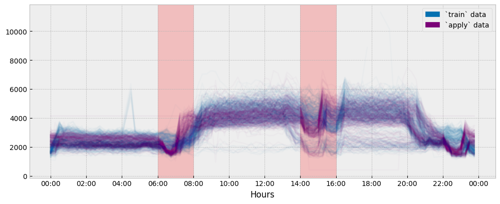
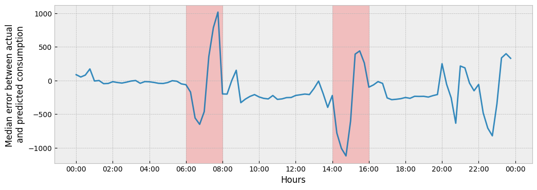
The plot suggests a significant misalignment in the occupancy patterns between the train and apply data during the hour intervals of 06:00-08:00 and 14:00-16:00. Let’s see if we are able to capture it:

change = y_apply["consumption"] - prediction # as consumption increase

change_daily = change.to_frame("change")
change_daily["date"] = change_daily.index.date
change_daily["time"] = change_daily.index.time

fig = plt.figure(figsize=(12, 4))
layout = (1, 1)
ax = plt.subplot2grid(layout, (0, 0))

change_daily.pivot(index='time', columns='date', values='change') \
            .mean(axis=1)                                      \
            .plot(ax=ax, alpha=0.8, legend=None, color='#0570b0')

ax.axvspan(time(6, 0), time(8, 0), alpha=0.2, color="red")
ax.axvspan(time(14, 0), time(16, 0), alpha=0.2, color="red")

ax.xaxis.set_major_locator(ticker.MultipleLocator(3600*2))
ax.set_xlabel('Hours')
ax.set_ylabel('Median error between actual \nand predicted consumption')

4.2.6. The predict pipeline with autoencoding

When run in the train namespace

Estimate activity levels for the train data:

for feature in X_train.columns:
    print(feature)

holiday
temperature

act_train = estimate_activity(
    X_train, 
    y_train, 
    non_occ_features="temperature", 
    exog="temperature",
    n_trials=200,
    verbose=False,
)

Then, fit a predictive model for the train data using the activity estimation as a feature, while removing occupancy related features:

X_train_act = pd.concat(
    [
        X_train.drop("holiday", axis=1),
        act_train.to_frame("activity")
        
    ], 
    axis=1
)

model = UsagePredictor(skip_calendar=True).fit(X_train_act, y_train)

When run in the apply namespace

Estimate activity:

act_apply = estimate_activity(
    X_apply, 
    y_apply, 
    non_occ_features="temperature", 
    exog="temperature",
    n_trials=200,
    verbose=False,
)

Apply the predictive model:

X_apply_act = pd.concat(
    [
        X_apply.drop("holiday", axis=1),
        act_apply.to_frame("activity")
    ], 
    axis=1
)

prediction = model.predict(X_apply_act)

Calculate the impact from the change:

change_auto = y_apply["consumption"] - prediction # as consumption increase

change_daily_auto = change_auto.to_frame("change")
change_daily_auto["date"] = change_daily_auto.index.date
change_daily_auto["time"] = change_daily_auto.index.time

The next plot shows the two impact estimations together:

fig = plt.figure(figsize=(12, 4))
layout = (1, 1)
ax = plt.subplot2grid(layout, (0, 0))

change_daily.pivot(index='time', columns='date', values='change') \
               .mean(axis=1)                                      \
               .plot(ax=ax, alpha=0.8, legend=None, color='#0570b0')

change_daily_auto.pivot(index='time', columns='date', values='change') \
               .mean(axis=1)                                      \
               .plot(ax=ax, alpha=0.8, legend=None, color='#fd8d3c')

ax.legend(
    [
        "Change estimation through prediction", 
        "Change estimation through autoencoding"
    ], 
    frameon=True
)

ax.axvspan(time(6, 0), time(8, 0), alpha=0.2, color="red")
ax.axvspan(time(14, 0), time(16, 0), alpha=0.2, color="red")

ax.xaxis.set_major_locator(ticker.MultipleLocator(3600*2))
ax.set_xlabel('Hours')
ax.set_ylabel('Average change in consumption')

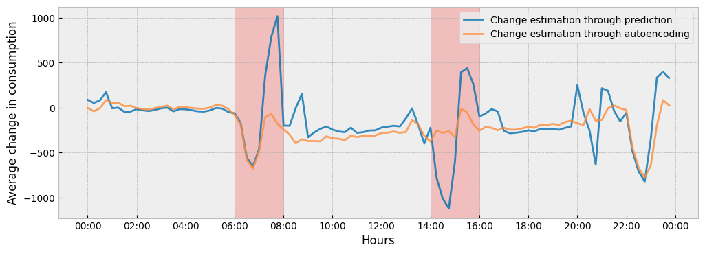
To understand the difference between the two (2) impact estimations, we can see how the estimated activity levels in train and apply periods differ from each other:

act_train_daily = act_train.to_frame("activity")
act_train_daily["date"] = act_train_daily.index.date
act_train_daily["time"] = act_train_daily.index.time

act_apply_daily = act_apply.to_frame("activity")
act_apply_daily["date"] = act_apply_daily.index.date
act_apply_daily["time"] = act_apply_daily.index.time

fig = plt.figure(figsize=(12, 4))
layout = (1, 1)
ax = plt.subplot2grid(layout, (0, 0))

act_train_daily.pivot(index='time', columns='date', values='activity') \
               .mean(axis=1)                                      \
               .plot(ax=ax, alpha=0.8, legend=None, color='#0570b0')

act_apply_daily.pivot(index='time', columns='date', values='activity') \
               .mean(axis=1)                                      \
               .plot(ax=ax, alpha=0.8, legend=None, color='#fd8d3c')

ax.legend(
    [
        "Activity estimation for `train` data", 
        "Activity estimation for `apply` data"
    ], 
    frameon=True
)

ax.axvspan(time(6, 0), time(8, 0), alpha=0.2, color="red")
ax.axvspan(time(14, 0), time(16, 0), alpha=0.2, color="red")

ax.xaxis.set_major_locator(ticker.MultipleLocator(3600*2))
ax.set_xlabel('Hours')
ax.set_ylabel('Average change in activity')

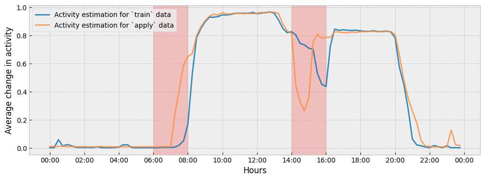
The autoencoding approach gives much less weight to changes in energy consumption that can be accounted for by changes in activity levels. For instance:

• There is a change in the activity levels during the hour interval of 07:00-08:00, so the impact that is estimated by the autoencoding approach during this interval will be lower than the impact estimated by the prediction-based approach.

• The autoencoding approach regards the change of energy consumption during the hour interval of 14:00-16:00 mainly as activity driven (a shift in activity levels) and, as a result, the counterfactual prediction for this interval is practically flat.

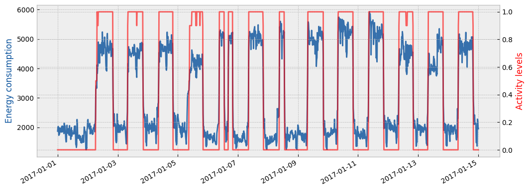
Finally, the following plot shows the estimated activity levels along with the actual energy consumption for the apply period and for the first two (2) weeks of January:

month = 1 # January
n_obs = 14*24*4

fig = plt.figure(figsize=(12, 4.5))
layout = (1, 1)
ax1 = plt.subplot2grid(layout, (0, 0))
ax2 = ax1.twinx()

y_apply["consumption"].loc[y_apply.index.month==month][:n_obs].plot(
    ax=ax1, color="#08519c", alpha=0.8
)
act_apply.loc[act_apply.index.month==month][:n_obs].plot(ax=ax2, color="red", alpha=0.6)


ax1.set_ylabel("Energy consumption", color="#08519c")
ax2.set_ylabel("Activity levels", color="red")
ax1.set_xlabel("")

4.3. Parameters

The relevant parameters - as they can be found in the eensight/conf/base/parameters/predict.yml file - are:

params = ConfigLoader(PROJECT_PATH / "conf").get("parameters*", "parameters*/**", "**/parameters*")

params = {
    "fit": params["fit"],
    "activity": params["activity"]
}

for name in ("assume_hurdle", "n_trials_adjust", "upper_bound"):
    params["activity"].pop(name)
    
params

{
    'fit': {'lags': {'temperature': [1, 2, 24]}, 'cat_features': 'holiday', 'validation_size': 0.2},
    'activity': {
        'non_occ_features': 'temperature',
        'cat_features': 'holiday',
        'exog': 'temperature',
        'n_trials': 200,
        'verbose': True
    }
}

---